5. Visualization of trees: annotation

This is also available as an R Script file: scripts_tree_operations.R

Prepare the data

Read a substitution table for tip labels. The first column must contain the same values as tips in the tree, the other column(s) - your pretty labels

labels <- read.csv('data/labels_simple.csv')

Combine tree and new labels. Similarly, you can plug in any kind of data you may want to plot, e.g. values of morphological traits. %<+% is a ggtree-specific operator working as a left join in SQL. It produces a treedata object:

tree_data <- ggtree(bayesTree_rooted) %<+% labels

In the same fashion add bootstrap values obtained with the getSupports function earlier. Note that it automatically maps bootstraps to the tree on the basis of node field shared between supportsTable and tree_data.

tree_data <- tree_data %<+% supportsTable

Plot the result

As before, separate geoms describe different sets of objects, and connected with a + sign.

• geom_tiplab shows labels from column label_pretty that was received from labels object.
• geom_label2 plots both posteriors and bootstraps with a use of concatenating paste function, with slash (/) as separator. Note the ifelse conditions that recognize missing values with is.na, and draw ‘-‘ on branches that did not appear in one of the trees. subset = !isTip here is needed to prevent the geom_label2 from plotting tip labels - they are already done.
• xlim is needed to fix truncation of long labels. You may need to change its second parameter or even drop xlim altogether, depending on your tree. Note that when plotting your tree with some additional data that do not fit into area specified by xlim, it may drop these data completely out of your plot.

  tree_data +
  geom_tiplab(aes(label = label_pretty), offset = 0.001) +
  geom_label2(
    aes(
      label = paste(
        ifelse(is.na(round(as.numeric(label), 2)),
        '-', round(as.numeric(label), 2)),
        ifelse(is.na(support),
               '-', support),
        sep = '/'
      ),
      subset = !isTip & label != 'Root'
    ),
    hjust = 1.1,
    vjust = -0.3,
    alpha = 0.8,
    label.size = NA,
    label.padding = unit(0.2, 'mm'),
    size = 2
  ) +
  xlim(0, 0.5)
  

Save the result

This function saves the last plotted graph. If you need to save a particular object, specify plot = object_name in ggsave.

## Create a directory for output files:
dir.create('output')

## Write the result
ggsave(
  filename = 'output/tree_data_lab.pdf',
  device = 'pdf',
  width = 210,
  height = 297,
  units = 'mm'
)

The main part is done, unless you want to play more with annotations or visualizations.

Bonus renaming

Read the table with more information on labels. Here we explicitly ask to read empty strings as NA value (na.strings = ''), so they will be properly parsed by is.na in plotting below. This will help to make labels look cleaner, without orphan commas.

labels_extended <- read.csv('data/labels_extended.csv', na.strings = '')

Add these data.

tree_data <- tree_data %<+% labels_extended

Plot the result. In this case we construct labels from separate fields using paste.

tree_data +
  geom_tiplab(
    aes(label = paste(
      label,
      ifelse(is.na(Organism),
             '', paste(',', Organism)),
      ifelse(is.na(Country),
             '', paste(',', Country)),
      ifelse(is.na(Altitude),
             '', paste(', altitude:', Altitude, 'm')),
      sep = ''
    )),
    geom = 'label',
    label.size = NA,
    label.padding = unit(0, 'mm'),
    offset = 0.001
  ) +
  geom_label2(
    aes(
      label = paste(
        ifelse(is.na(round(as.numeric(label), 2)),
        '-', round(as.numeric(label), 2)),
        ifelse(is.na(support),
               '-', support),
        sep = '/'
      ),
      subset = !isTip & label != 'Root'
    ),
    hjust = 1.1,
    vjust = -0.3,
    alpha = 0.8,
    label.size = NA,
    label.padding = unit(0.2, 'mm'),
    size = 2
  ) +
  xlim(0, 0.5)

Save the result.

ggsave(
  filename = 'output/tree_data_lab_ext.pdf',
  device = 'pdf',
  width = 420,
  height = 297,
  units = 'mm'
)

Bonus highlighting clades

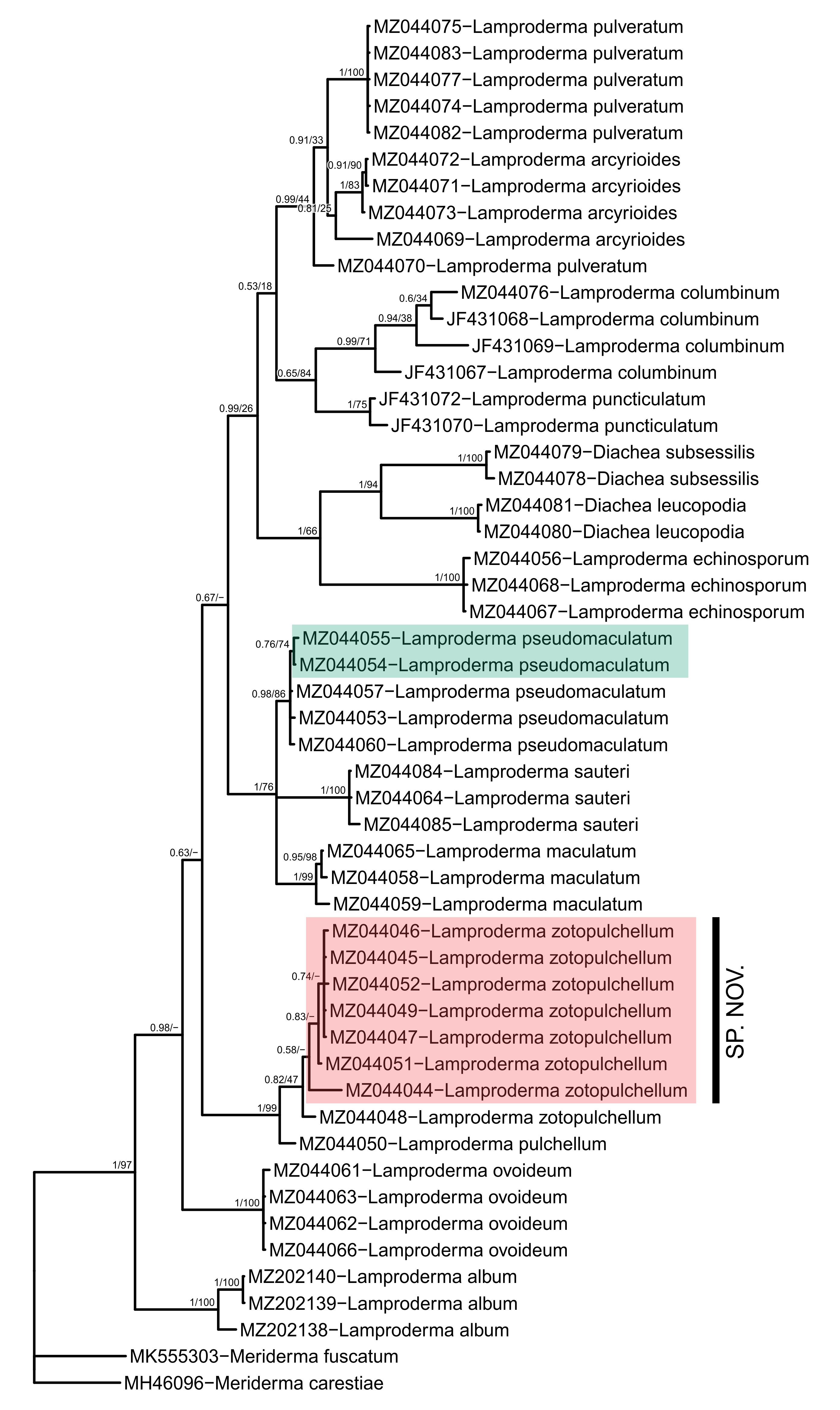
For this purpose ggtree provides several geoms, e.g. geom_hilight, geom_balance (see again https://yulab-smu.top/treedata-book/chapter5.html). With geom_cladelabel we additionally can delineate clades with labeled vertical bars. We will highlight 2 clades and add 1 labelled bar by adding these geometries to the code. Note that order in which we lay out geoms defines their rendering order: e.g. here highlights will be drawn under tip labels to keep the latter untinted, black.

tree_data +
  geom_label2(
    aes(
      label = paste(
        ifelse(is.na(round(as.numeric(label), 2)),
               '-', round(as.numeric(label), 2)),
        ifelse(is.na(support),
               '-', support),
        sep = '/'
      ),
      subset = !isTip & label != 'Root'
    ),
    hjust = 1.1,
    vjust = -0.3,
    alpha = 0.8,
    label.size = NA,
    label.padding = unit(0.2, 'mm'),
    size = 2
  ) +
  geom_hilight(node = 65, fill="#1B9E77", alpha = 0.3, extend = 0.22) + 
  geom_hilight(node = 56, fill="#F54748", alpha = 0.3, extend=0.20) +
  geom_cladelabel(56, "SP. NOV.", offset = 0.12, barsize = 2, align = TRUE, angle = 90, offset.text = 0.008, extend = 0.5, hjust = 0.5, fontsize=5) +
  geom_tiplab(aes(label = label_pretty), offset = 0.001)  +
  xlim(0, 0.5)

Save the result.

ggsave(
  filename = 'output/tree_data_highlighted.pdf',
  device = 'pdf',
  width = 210,
  height = 297,
  units = 'mm'
)

Example of an ouput:

That’s all for now, folks!

Home